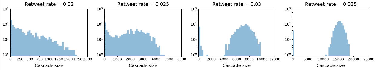
Is the final size of a large-scale information cascade predictable?
The cascade size distributions obtained with online social network (OSN)
simulations suggest that predicting an approximate size is not infeasible.
This is because as the retweet rate increases, cascades split more clearly
into tiny and large cascade groups, and the coefficient of variation of
cascade sizes of the large cascade group decreases.
Histograms of the final sizes of Twitter-type information cascades over
scale-free random networks.
Reproduction of bi-polarization
The following describes the recurrence relation (RR) model that is designed to reproduce the bi-polarization phenomenon described above.
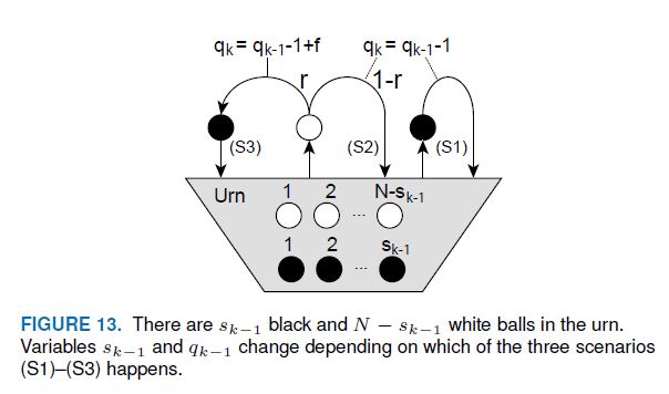
Fig. 13 illustrates the RR model. There are N balls in an urn, and they
are either white or black.
Here, the term trial indicates a process of drawing a ball randomly from
the urn and returning a ball to the urn.
The model has two state variables. Variable sk represents the number of black balls in the urn immediately after the
k-th trial, and qk is the number of remaining trials.
At each trial k(= 0, 1, ...), there are three scenarios (S1)-(S3) after
one ball is drawn from the urn.
(S1) If the drawn ball is black (which occurs with probability sk-1/N), it is placed back in the urn; otherwise, with probability 1-r, (S2)
the ball is returned to the urn, and, with probability r, (S3) a black
ball is placed in the urn and qk is obtained by adding f to qk-1-1.
In other words, scenarios (S1) and (S2) change the variables as
sk = sk-1,
qk = qk-1-1,
and in the case of (S3),
sk = sk-1+1,
qk = qk-1-1 + f.
The RR begins with s0 = 0 and q0 = f0, and terminates when qk becomes zero.
A Mathematica program for calculating {sk, qk} can be found at the end of this page.
The RR model is a simplification of the OSN simulation model in the paper.
All balls in the urn represent OSN users, and a black (white) ball denotes an adopter (nonadopter), where an adopter (nonadopter) is a user who has (not) retweeted.
Variables r and f correspond to the retweet probability and the number
of followers, respectively.
In Fig. 13, (S1) an adopter never retweets.
(S2) A nonadopter decides not to post a retweet with probability 1 − r, and (S3) a nonadopter decides to post it with probability r.
The probability that an adopter (nonadopter) makes a decision is sk−1/N (1 − sk−1/N).
(S1) and (S2) ((S3)) represent the state change after a user decides (not) to retweet, where qk can be considered as the number of messages awaiting user decisions.
The initial value q0 = f0 implies that the initiator has f0 followers.
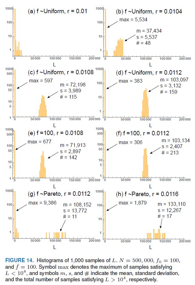
Fig. 14 shows histograms of L when N = 500, 000, f0 =100, and f = 100, where L denotes sk at qk = 0 (i.e., L represents the final cascade size), and f is the mean of the distribution of f.
Figs. 14(a)–(d) present the cases where f has a uniform distribution U(1,
199).
These figures suggest that bi-polarization occurs when r f exceeds 1.
Figs. 14(e)–(f) present the histograms obtained when f is fixed at 100.
Figs. 14(e) and 14(f) are very similar to Figs. 14(c) and 14(d), respectively.
Figs. 14(g)–(h) exhibit the cases where f has a truncated Pareto distribution
with (a, b) = (0.5, 103), where the distribution is given by f(t;a,b)=(1-t-a)/(1-(1/b)a).
The figures illustrate that the emergence of bi-polarization requires a
larger r.
The mechanisms of generating bi-polarization included in the RR and OSN
models may be the same because bi-polarization shown in Figs. 14(b)-(h)
indicates the following three features that can also be observed in the
results of the OSN model.
1) Most of the samples in the small L group are distributed around zero;
the small (large) L group is defined as a group of samples satisfying L
< 104 (L > 104).
2) The size of the large L group (denoted by # in Fig. 14) increases with
r.
3) The CV of the large L group decreases with an increase in r because
its standard deviation (denoted by s in Fig. 14) decreases slightly as
r increases.